SciPy - PeP et al. Toolbox Workshop

Baut auf NumPy auf
Kann numerisch integrieren, DGLs lösen, optimieren, minimieren, …
Enthält auch physikalische Konstanten und wichtige mathematische Funktionen

Überblick über (fast) alles Weitere, was SciPy kann, gibt es hier:

scipy.ipynb

Inhalt¶

Abrufen von Naturkonstanten¶

Wenn solche Konstanten genutzt werden, muss das korrekt mitgeteilt, also zitiert werden. Darauf gehen wir nächste Woche im LaTeX-Workshop ein :-)

(Quelle hier: scipy + version)

import numpy as np

# physical constants
import scipy.constants as const

planck_value = const.Planck  # returns the value
planck_full = const.physical_constants[
    "Planck constant"
]  # returns value, unit and uncertainty
print(f"{planck_value = }", f"{planck_full = }", sep="\n")

planck_value = 6.62607015e-34
planck_full = (6.62607015e-34, 'J Hz^-1', 0.0)

# a list of all included constants
# search the web for "scipy physical constants reference guide" to find the same list
# We don't print the full list in the html file, to keep the notebook more managable
# const.physical_constants

# convert temperatures:
print(const.convert_temperature(100, "c", "K"))
print(const.convert_temperature(100, "kelvin", "Celsius"))
print(const.convert_temperature(100, "f", "C"))

373.15
-173.14999999999998
37.77777777777777

# convert angles:
print(np.rad2deg(np.pi))
print(np.deg2rad(90))

180.0
1.5707963267948966

Fitten¶

Oft möchte man eine Funktion mit freien Parametern, zum Beispiel eine Erwartung aus der Theorie, an die gemessenen Werte anpassen. Dies nennt man Fit.

Die Funktion scipy.optimize.curve_fit nutzt die numerische Methode der kleinsten Quadrate, die arbiträre Funktionen fitten kann. Für Funktionen, die eine Linearkombination von Einzelfunktionen sind, also

f(x) = \sum_i^N a_i \cdot f_i(x),

existiert eine analytische Lösung. Deswegen sollten in solchen Fällen (z.B. alle Polynome) entsprechende Funktionen genutzt werden (z.B. np.polyfit).

Lineare Regression bzw. Regression von Polynomen¶

Im Folgenden wird eine lineare Regression mit np.polyfit durchgeführt:

f(x) = a + b \cdot x

# prepare plot
%matplotlib inline
import matplotlib.pyplot as plt

plt.rcParams["figure.figsize"] = (10, 8)
plt.rcParams["font.size"] = 16

# load data
x, y = np.genfromtxt("data/example_data_linear.txt", unpack=True)

fig, ax = plt.subplots(1, 1, layout="constrained")

ax.plot(x, y, "k.", label="example data")
ax.set(xlabel=r"$t \,/\, \mathrm{s}$", ylabel=r"$s \,/\, \mathrm{m}$");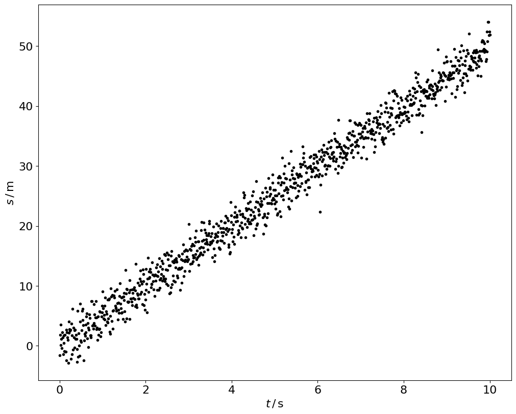

# Fit a polynomial of degree 1, return covariance matrix
params, covariance_matrix = np.polyfit(x, y, deg=1, cov=True)

uncertainties = np.sqrt(np.diag(covariance_matrix))

for name, value, uncertainty in zip("ab", params, uncertainties):
    print(f"{name} = {value:.3f} ± {uncertainty:.3f}")

a = 4.977 ± 0.021
b = 0.070 ± 0.124

x_plot = np.linspace(0, 10)

fig, ax = plt.subplots(1, 1, layout="constrained")

ax.plot(x, y, "k.", label="Messwerte")
ax.plot(
    x_plot,
    params[0] * x_plot + params[1],
    label="Lineare Regression",
    linewidth=3,
    color="tab:orange",
)
ax.legend()
ax.set(xlabel=r"$t \,/\, \mathrm{s}$", ylabel=r"$s \,/\, \mathrm{m}$");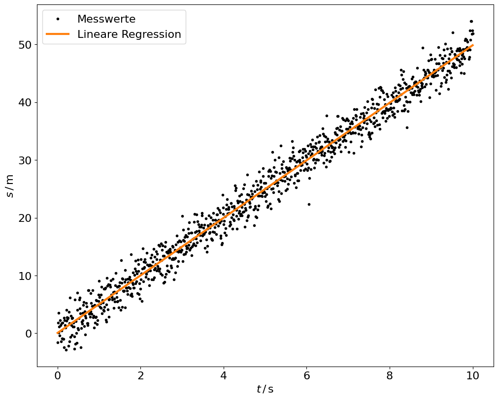

Nichtlineare Funktionen der Parameter¶

Wenn eine Funktion nicht linear bezüglich der freien Parameter ist, muss die Lösung numerisch gefunden werden.

Als erstes Beispiel dafür schauen wir uns folgende Daten an:

x, y = np.genfromtxt("data/sin_fit.txt", unpack=True)

ax.cla()

ax.plot(x, y, "o", label="Messwerte")
ax.set(xlabel=r"$t$ / s", ylabel=r"$U$ / V")
ax.legend()
fig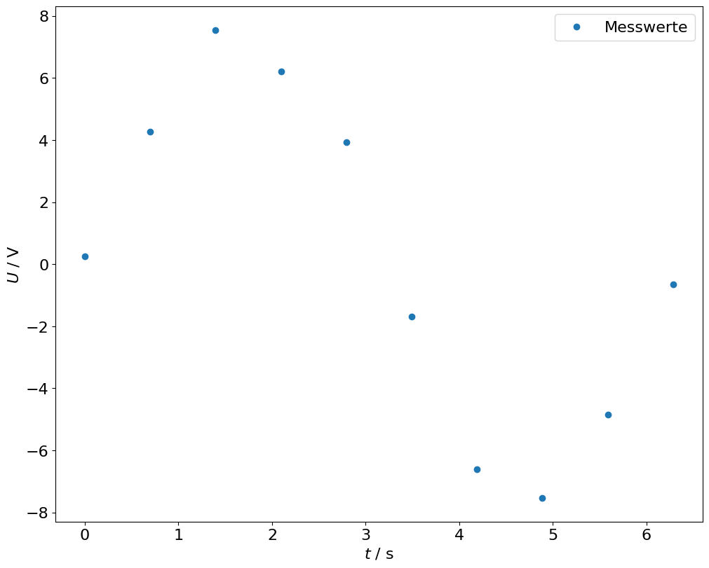

Diese Daten sollen an in der Theorie eine Sinus-Kurve beschreiben. Wir schreiben den Sinus allgemein als

U(t) = a \cdot \sin(b \cdot t) + c~.

und definieren uns die entsprechende Funktion im Code.

def sinus(x, a, b, c):
    return a * np.sin(b * x) + c

Für das fitten nutzen wir jetzt curve_fit und bekommen wieder die Parameter und Kovarianz-Matrix als Rückgabewerte.

from scipy.optimize import curve_fit

params, covariance_matrix = curve_fit(sinus, x, y)

uncertainties = np.sqrt(np.diag(covariance_matrix))

for name, value, uncertainty in zip("abc", params, uncertainties):
    print(f"{name} = {value:.3f} ± {uncertainty:.3f}")

a = 7.458 ± 0.255
b = 0.982 ± 0.008
c = 0.128 ± 0.172

Jetzt können wir die gefittete Funktion in den Plot der Messwerte hinzufügen.

ax.cla()

x_sin_fit = np.linspace(0, 2 * np.pi)

ax.plot(x, y, "o", label="Messwerte")
ax.plot(x_sin_fit, sinus(x_sin_fit, *params), label="Sinus Fit")
ax.set(xlabel=r"$t$ / s", ylabel=r"$U$ / V")
ax.legend()
fig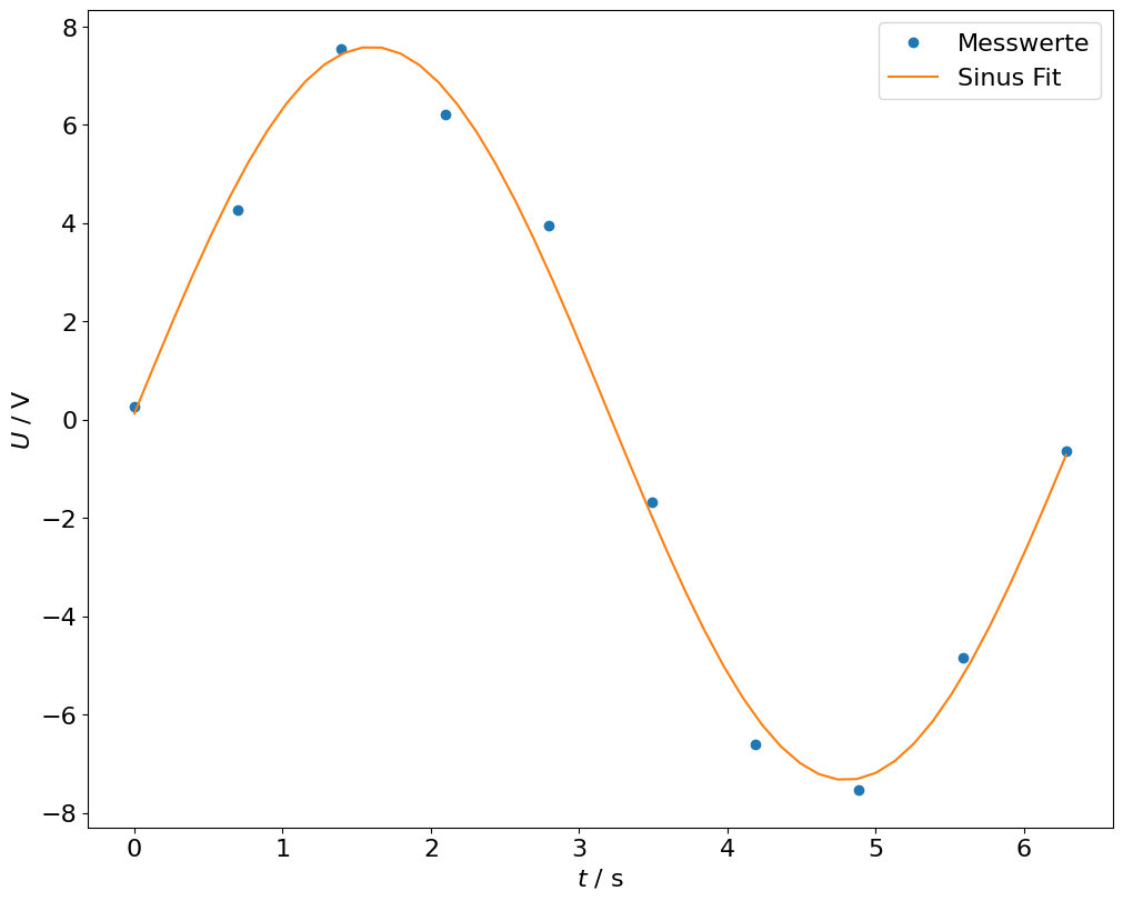

Bei dieser Variante des Fits kann es passieren, dass der Minimierungsalgorithmus in lokale Maxima hineinläuft und unsinnige Ergebnisse liefert, dies kann mit guten Startwerten meistens vermieden werden.

Als Beispiel einer komplexeren Funktion wird im Folgenden die Sigmoidfunktion verwendet (ähnlich zum tanh):

f(x; a, b, c) = \frac{a}{1 + \exp(-(x-b))} + c

def sigmoid(x, a, b, c):
    return a / (1 + np.exp(-(x - b))) + c


x_plot = np.linspace(-50, 50, 1000)

ax.cla()

ax.set_xlabel("x")
ax.set_ylabel("y")

ax.plot(x_plot, sigmoid(x_plot, 1, 0, 0), label="Sigmoid")
ax.plot(x_plot, np.tanh(x_plot), label="tanh")
ax.legend()
ax.set(xlabel=r"$x$", ylabel=r"$f(x)$")
fig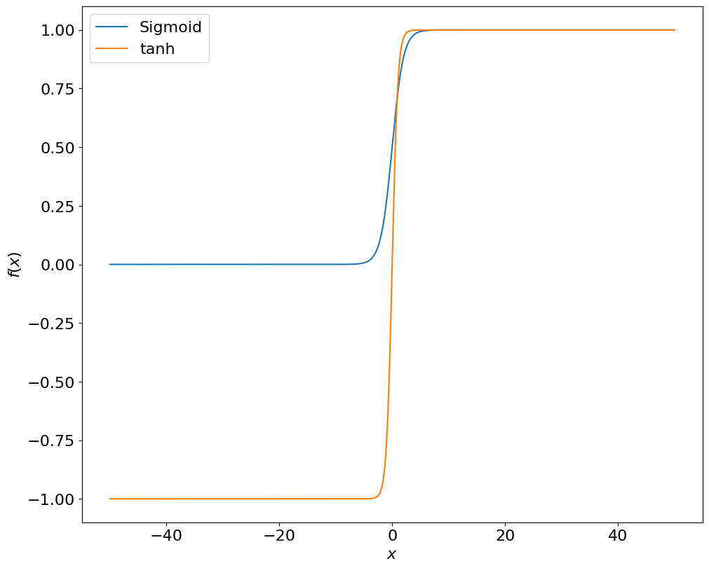

Die Messwerte aus einem Praktikumsversuch:

x, y = np.loadtxt("data/fit_data_with_init_values.txt", unpack=True)

ax.cla()
ax.plot(x, y, "o", label=r"Messwerte")

ax.set(xlabel=r"Temperatur / °C", ylabel=r"$GP$")
fig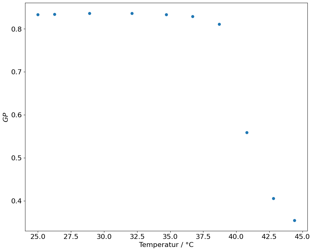

Ein einfacher Fit wie oben funktioniert hier nicht so gut:

params, covariance_matrix = curve_fit(sigmoid, x, y)

uncertainties = np.sqrt(np.diag(covariance_matrix))

for name, value, uncertainty in zip("abc", params, uncertainties):
    print(f"{name} = {value:8.3f} ± {uncertainty:.3f}")

a = -307.054 ± inf
b =    1.000 ± inf
c =  307.767 ± inf

/tmp/ipykernel_41925/1664943109.py:1: OptimizeWarning: Covariance of the parameters could not be estimated
  params, covariance_matrix = curve_fit(sigmoid, x, y)

Schaut man sich die berechnete Ausgleichskurve an sieht man auch, dass das nicht stimmen kann:

ax.cla()

ax.plot(x, y, "o", label="Messdaten")
ax.plot(x_plot, sigmoid(x_plot, *params), "-", label=r"Sigmoid Fit")

ax.legend()
ax.set(xlabel=r"Temperatur / °C", ylabel=r"$GP$")

axins = ax.inset_axes(
    [0.60, 0.4, 0.3, 0.3],
    xlim=(24, 46), ylim=(0.3, 0.9)
)
axins.plot(x, y, "o")
axins.plot(x_plot, sigmoid(x_plot, *params), "-")
ax.indicate_inset_zoom(axins, edgecolor="black", alpha=0.4)

fig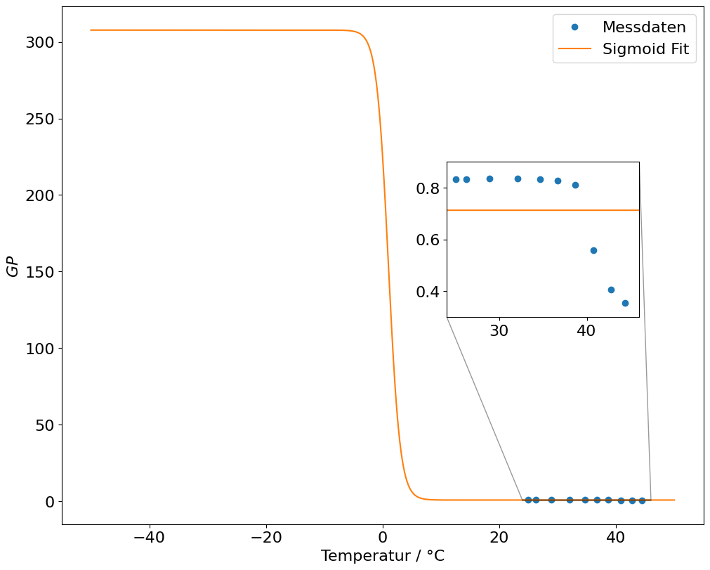

Was macht man jetzt?
Bei solchen Fragen hilft die Dokumentation der Pythonmodule (hier: scipy) oder Stack Overflow weiter.
Folgendes Google-Muster ist ein guter Anfang (beachte englische Sprache):

python <module-name> <function-name> <What went wrong?>

Also in diesem Fall: python scipy curve_fit fails

Damit dieser Fit funktioniert müssen die Startwerte für den internen Minimierungsalgorithmus angepasst werden.
Aus der Dokumentation/Stack Overflow wissen wir jetzt, dass man mit dem keyword argument p0 (Standardwert is p0=(1,1,1)) die Startwerte einstellt:

params, covariance_matrix = curve_fit(sigmoid, x, y, p0=(-1, 40, 1))


uncertainties = np.sqrt(np.diag(covariance_matrix))

for name, value, uncertainty in zip("abc", params, uncertainties):
    print(f"{name} = {value:8.3f} ± {uncertainty:.3f}")

a =   -0.494 ± 0.014
b =   40.668 ± 0.137
c =    0.839 ± 0.006

ax.cla()
x_plot = np.linspace(0, 50, 1000)

ax.plot(x, y, "o", label="Messwerte")
ax.plot(x_plot, sigmoid(x_plot, *params), "-", label="Sigmoid Fit")

ax.legend()
ax.set(xlabel=r"Temperatur / °C", ylabel=r"$GP$")
fig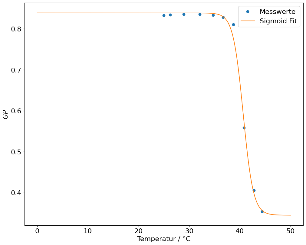

Zum Vergleich der beiden Anfangswerte (seeds) kann man sich die einmal ansehen und mit den angepassten Parametern vergleichen:

default_seed = (1, 1, 1)
good_seed = (-1, 40, 1)

parameter = [default_seed, good_seed, params]

x_plot = np.linspace(-80, 80, 1000)

ax.cla()
for a, b, c in parameter:
    ax.plot(
        x_plot, sigmoid(x_plot, a, b, c), label=f"f(x; {a:0.3f}, {b:0.3f}, {c:0.3f})"
    )

ax.legend()
ax.set(xlabel=r"$x$", ylabel=r"$f(x)$")
fig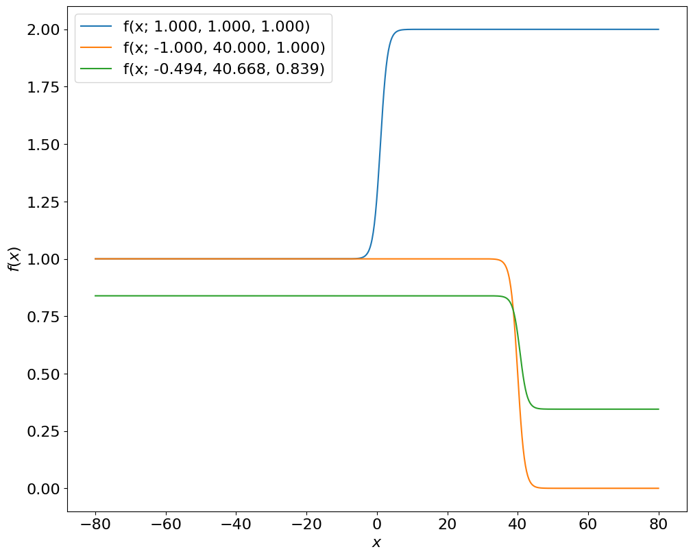

Die richtigen Startwerte findet man entweder durch

trial and error => einfach ausprobieren bis es klappt
nachdenken => siehe unten

Im obigen Beispiel musste nur der Parameter b angepasst werden, weil der für die Form der Kurve sehr wichtig ist.

f(x; a, b, c) = \frac{a}{1 + \exp(-(x-b))} + c

bs = [0, 20, 40]

x_plot = np.linspace(-50, 50, 1000)

ax.cla()


for b in bs:
    (line,) = ax.plot(x_plot, sigmoid(x_plot, 1, b, 0), label=f"f(x; 1, {b}, 0)")

    ax.plot(
        b,
        sigmoid(b, 1, b, 0),
        "o",
        color=line.get_color(),
        ms=20,
        label=f"f(x={b}) = {sigmoid(b, 1, b, 0)}",
    )


ax.legend()
ax.set(xlabel=r"$x$", ylabel=r"$f(x)$")
fig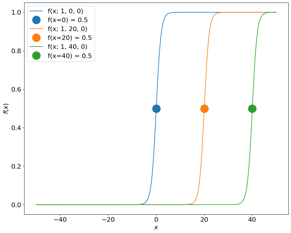

Der Parameter $b$ gibt den $x$ -Wert an, bei dem die Funktion auf die Hälfte des Maximums abgefallen ist.
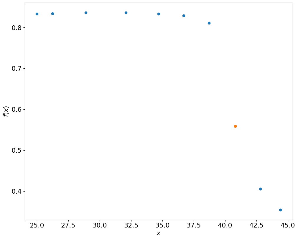
Bei den Messwerten oben ist die Stelle ungefähr bei $x=40$ , also ist b = 40 ein guter Startwert.

Das lässt sich auch automatisieren:

ax.cla()
ax.plot(x, y, "o")

idx = np.argmin(np.abs(y - 0.5))

ax.plot(x[idx], y[idx], "o")

print(x[idx], y[idx])
ax.set(xlabel=r"$x$", ylabel=r"$f(x)$")
fig

40.8 0.5586250642

Weitere nützliche Funktionen für das Praktikum¶

Folgende Eigenschaften von Scipy sollen nur die Idee vermitteln, was noch alles möglich ist.

Statistische Verteilungen und Funktionen¶

Das scipy.stats Modul enthält viele Wahrscheinlichkeitsverteilungen und -funktionen. Als Beispiel wird hier jedoch nur die Standardabweichung des Mittelwertes berechnet.

import numpy as np

x = np.array([2, 5, 7])  # create test array

from scipy.stats import sem

print(sem(x))  # standard error of the mean

1.4529663145135578

Finden von Peaks¶

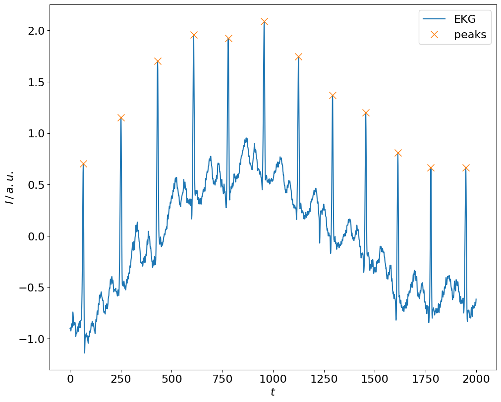
Das scipy.signal Modul enthält Funktionen zur Signalverarbeitung. Das kann interessant sein zum automatischen Finden von Peaks, oder Bestimmung der Periodizität.

# example data
from scipy.datasets import electrocardiogram

x = electrocardiogram()[2000:4000]

# find peaks
from scipy.signal import find_peaks

peaks, _ = find_peaks(x, distance=150)

fig, ax = plt.subplots(1, 1, layout="constrained")

ax.plot(x, label="EKG")
ax.plot(peaks, x[peaks], "x", ms=10, label="peaks")
ax.set(xlabel=r"$t$", ylabel=r"$I \,/\, a.u.$")
ax.legend();