Automatisieren von Fehlerrechnung

Gesucht: Unsicherheit von $f(x_1, \dots x_m)$ , wenn $x_i$ Unsicherheiten haben
Gaußsche Fehlerfortpflanzung:

\sigma_{f} = \sqrt{\sum_{i=1}^m \left( \frac{\partial f}{\partial x_i}\right)^{\!2} \sigma_{x_i}^2}

Manuelle Fehlerfortpflanzung:

Berechne die Ableitungen von $f$ nach allen fehlerbehafteten Größen $x_i$
Ableitungen in die obere Formel einsetzen
Werte und Unsicherheiten der $x_i$ einsetzen

Probleme:
Kompliziert, dauert lange, man macht oft Fehler
Falsches Ergebnis, wenn $x_i$ korreliert sind, dann erweiterte Fehlerfortpflanzung:

\sigma_{f} = \sqrt{\sum_{i=1}^m \left( \frac{\partial f}{\partial x_i}\right)^{\!2} \sigma_{x_i}^2 + \sum_{j\neq k} \frac{\partial f}{\partial x_j} \frac{\partial f}{\partial x_k} \operatorname{cov}(x_j, x_k)}

$\operatorname{cov}(x_j, x_k)$ sind die Einträge der Kovarianzmatrix und beschreiben die Korrelation zwischen den Unsicherheiten von $x_j$ und $x_k$
konkret für zwei Messgrößen x, y, die $N$ mal gemessen wurden:

\operatorname{cov}(x, y) = \frac{\sum_{i = 1}^{N} (x_i - \bar{x})(y_i - \bar{y})}{N}

`uncertainties`¶

Erlaubt es, Fehlerrechnung automatisch durchzuführen
Datentyp: ufloat, repräsentiert Wert mit Unsicherheit

from uncertainties import ufloat

x = ufloat(5, 1)
y = ufloat(3, 1)

x + y

8.0+/-1.4142135623730951

Korrelationen werden von uncertainties beachtet:

x = ufloat(3, 1)
y = ufloat(3, 1)

print(x - y)
print(x - x)  # error is zero!

print(x == y)

0.0+/-1.4
0.0+/-0
False

uncertainties.unumpy ergänzt numpy:

import numpy as np
import uncertainties.unumpy as unp

x = [1, 2, 3, 4, 5]
err = [0.1, 0.3, 0.1, 0.8, 1.0]

y = unp.uarray(x, err)

unp.cos(unp.exp(y))

array([-0.9117339147869651+/-0.11166193174450133,
       0.4483562418187328+/-1.9814233218473645,
       0.3285947554325321+/-1.8970207322669204,
       -0.3706617333977958+/-40.567208903209576,
       -0.7260031145123346+/-102.06245489729305], dtype=object)

Man muss daran denken, jetzt die Funktionen aus unumpy zu benutzen (exp, cos, etc.).

np.cos(x)

array([ 0.54030231, -0.41614684, -0.9899925 , -0.65364362, 0.28366219])

Zugriff auf Wert und Standardabweichung mit n und s:

x = ufloat(5, 1)
print(x.n)
print(x.s)

5.0
1.0

Bei unumpy mit nominal_values und std_devs

x = unp.uarray([1, 2, 3], [0.3, 0.3, 0.1])
print(unp.nominal_values(x))
print(unp.std_devs(x))

[1. 2. 3.]
[0.3 0.3 0.1]

Kann man natürlich auch im import abkürzen:

from uncertainties.unumpy import nominal_values as noms, std_devs as stds

print(noms(x))
print(stds(x))

[1. 2. 3.]
[0.3 0.3 0.1]

Korrelierte Werte¶

import numpy as np
import matplotlib.pyplot as plt

plt.rcParams["figure.figsize"] = (8, 4)
plt.rcParams["font.size"] = 16

x = np.array([90, 60, 45, 100, 15, 23, 52, 30, 71, 88])
y = np.array([90, 71, 65, 100, 45, 60, 75, 85, 100, 80])

fig, ax = plt.subplots(1, 1, layout="constrained")

ax.plot(x, y, "ro")
ax.set_xlabel("x")
ax.set_ylabel("y");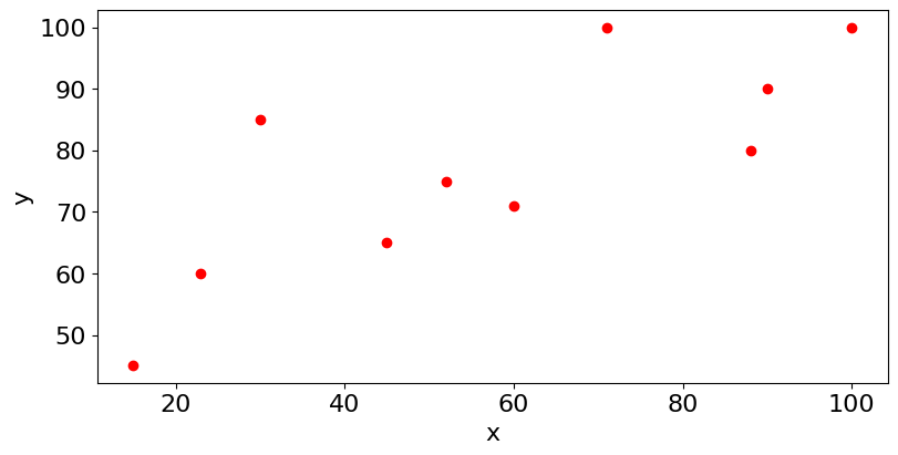

Wir vermuten eine lineare Korrelation der Messwerte und stützen die Hypothese mit dem Korrelationskoeffizient:

r = \frac{cov(x, y)}{\sigma_x \sigma_y}, \quad -1 \leq r \leq 1

x_mean = np.mean(x)
y_mean = np.mean(y)

dx = x - x_mean
dy = y - y_mean
corr_coeff = np.sum(dx * dy) / np.sqrt(np.sum(dx**2) * np.sum(dy**2))
print(corr_coeff)

0.7807249232806309

Korrelation zwischen Variablen mit correlated_values erzeugen:

from uncertainties import correlated_values

values = [1, 2]

cov = [[0.5, 0.25], [0.25, 0.2]]

x, y = correlated_values(values, cov)

Vorsicht bei Fits:¶

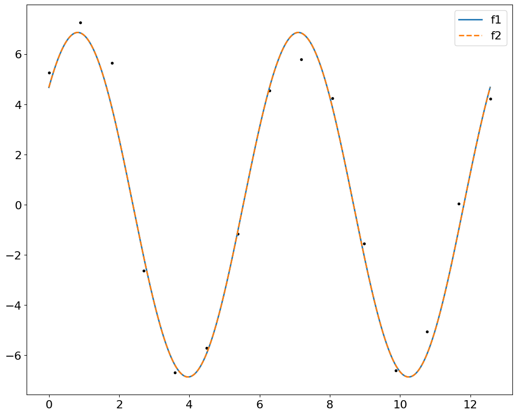
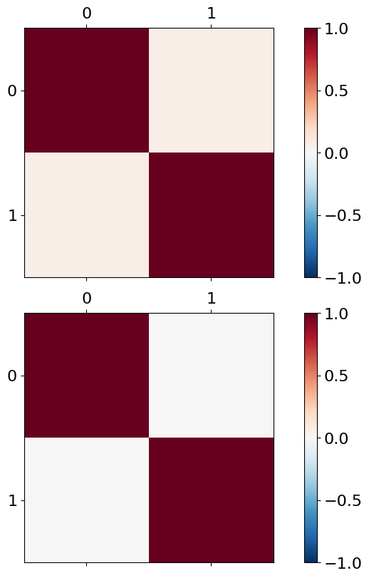
Korrelierte Fit-Parameter führen zu nichts-sagenden Ergebnissen. Kontrolle: Korrelationsmatrix.

%matplotlib inline

import numpy as np
import matplotlib.pyplot as plt

plt.rcParams["figure.figsize"] = (10, 8)
plt.rcParams["font.size"] = 16
from scipy.optimize import curve_fit
from uncertainties import correlated_values, correlation_matrix

rng = np.random.default_rng()


def f1(x, a, phi):
    return a * np.cos(x + phi)


def f2(x, a, b):
    return a * np.cos(x) + b * np.sin(x)


x = np.linspace(0, 4 * np.pi, 15)
y = 5 * np.sin(x) + 5 * np.cos(x) + rng.normal(0, 0.8, 15)

params1, cov1 = curve_fit(f1, x, y)
params2, cov2 = curve_fit(f2, x, y)

params1 = correlated_values(params1, cov1)
params2 = correlated_values(params2, cov2)


x_plot = np.linspace(0, 4 * np.pi, 1000)

fig, ax = plt.subplots(1, 1, layout="constrained")

ax.plot(x, y, "k.")

ax.plot(x_plot, f1(x_plot, *noms(params1)), label="f1", lw=2)
ax.plot(x_plot, f2(x_plot, *noms(params2)), "--", label="f2", lw=2)

ax.legend()

fig, (ax1, ax2) = plt.subplots(2, 1, layout="constrained")

print(correlation_matrix(params1))
print(correlation_matrix(params2))

mat1 = ax1.matshow(correlation_matrix(params1), cmap="RdBu_r", vmin=-1, vmax=1)
mat2 = ax2.matshow(correlation_matrix(params2), cmap="RdBu_r", vmin=-1, vmax=1)
fig.colorbar(mat1, ax=ax1)
fig.colorbar(mat2, ax=ax2);

[[1.         0.06649402]
 [0.06649402 1.        ]]
[[ 1.00000000e+00 -1.97072984e-09]
 [-1.97072984e-09  1.00000000e+00]]

Vorsicht¶

Man kann keine ufloats plotten:

x = np.linspace(0, 10)
y = unp.uarray(np.linspace(0, 5), 1)

fig, ax = plt.subplots(1, 1, layout="constrained")

# ax.plot(x, y, 'rx')
ax.errorbar(x, unp.nominal_values(y), yerr=unp.std_devs(y), fmt="rx");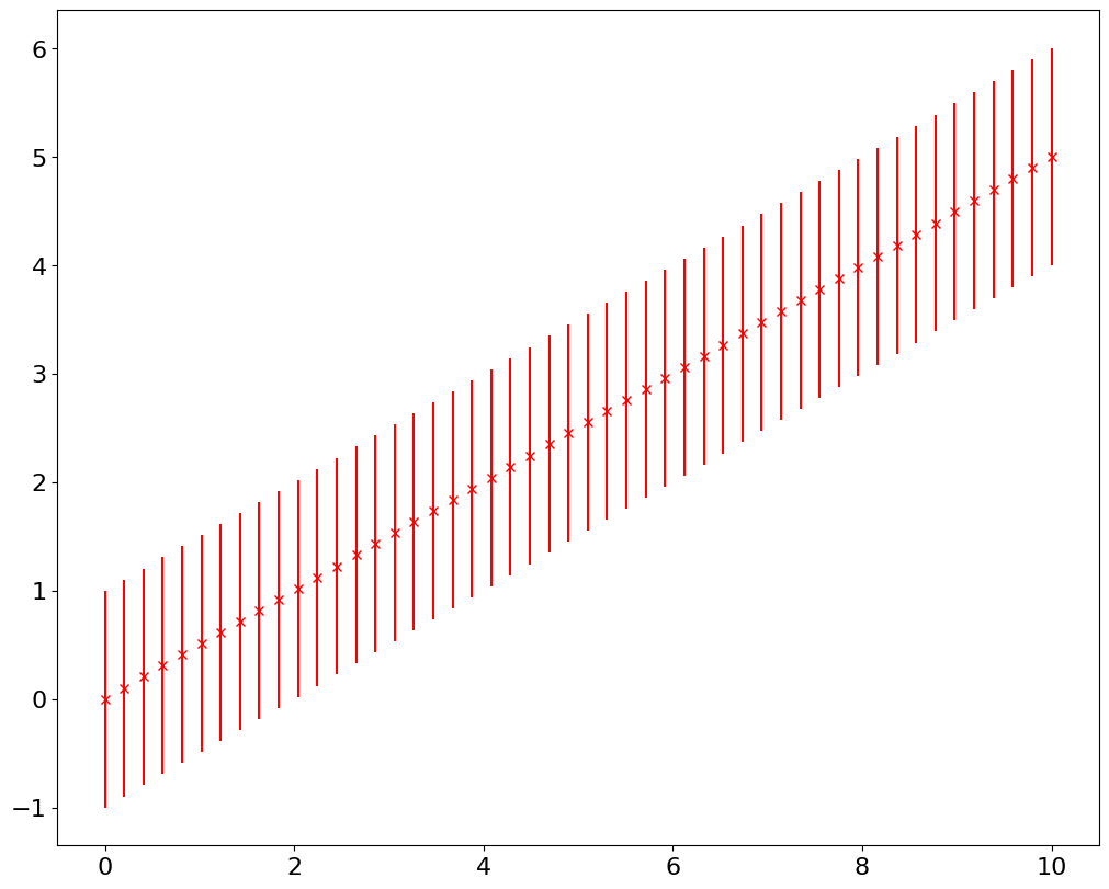

SymPy¶

Kann Ableitungen automatisch generieren

SymPy importieren:

import sympy

Mathematische Variablen erzeugen mit var():

x, y, z = sympy.var("x y z")

x + y + z

Differenzieren mit diff():

f = x + y**3 - sympy.cos(z) ** 2

print(f)
print(f.diff(x))
print(f.diff(y))
print(f.diff(z))
print(f.diff(z, z, z))

x + y**3 - cos(z)**2
1
3*y**2
2*sin(z)*cos(z)
-8*sin(z)*cos(z)

Eine Funktion, die automatisch die Fehlerformel generiert:

import sympy


def error(f, err_vars=None):
    from sympy import Symbol, latex

    s = 0
    latex_names = dict()

    if err_vars is None:
        err_vars = f.free_symbols

    for v in err_vars:
        err = Symbol("latex_std_" + v.name)
        s += f.diff(v) ** 2 * err**2
        latex_names[err] = "\\sigma_{" + latex(v) + "}"

    return latex(sympy.sqrt(s), symbol_names=latex_names)


E, q, r = sympy.var("E_x q r")

f = E + q**2 * r

print(f)
print(error(f))
print()

E_x + q**2*r
\sqrt{\sigma_{E_{x}}^{2} + 4 \sigma_{q}^{2} q^{2} r^{2} + \sigma_{r}^{2} q^{4}}

f= E + q^2 r \quad\rightarrow\quad \sigma_f = \sqrt{\sigma_{E_{x}}^{2} + 4 \sigma_{q}^{2} q^{2} r^{2} + \sigma_{r}^{2} q^{4}}

uncertainties¶

Korrelierte Werte¶

Vorsicht bei Fits:¶

Vorsicht¶

SymPy¶

`uncertainties`¶